One of my first baby steps into the open source world, was when I answered this SO question over four years ago. Recently I revisited the post and saw that Z.Lin did a very nice and more modern implementation, using dplyr and facetting in ggplot2. I decided to merge here ideas with mine to create a general function that makes MM plots. I also added two features: counts, proportions, or percentages to the cells as text and highlighting cells by a condition.
For those of you unfamiliar with this type of plot, it graphs the joint distribution of two categorical variables. x is plotted in bins, with the bin widths reflecting its marginal distribution. The fill of the bins is based on y. Each bin is filled by the co-occurence of its x and y values. When x and y are independent, all the bins are filled (approximately) in the same way. The nice feature of the MM plot, is that is shows both the joint distribution and the marginal distributions of x and y.
ggmm
To demonstrate the function, I’ll take a selection of the emergency data set from the padr package. Such that it has three types of incidents in four parts of town. We also do some relabelling for prettier plot labels.
em_sel <- padr::emergency %>% dplyr::filter(
  title %in% c("Traffic: VEHICLE ACCIDENT -", "Traffic: DISABLED VEHICLE -", "Fire: FIRE ALARM"),
  twp   %in% c("LOWER MERION", "ABINGTON", "NORRISTOWN", "UPPER MERION")) %>%
  mutate(twp = factor(twp,
                      levels = c("LOWER MERION", "ABINGTON", "NORRISTOWN", "UPPER MERION"),
                      labels = c("Low Mer.", "Abing.", "Norris.", "Upper Mer.")))
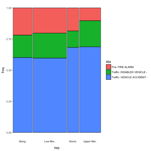
The function takes a data frame and the bare (unquoted) column names of the x and y variables. It will then create a ggplot object. The variables don’t have to be factors or characters, the function coerces them to character.
ggmm(em_sel, twp, title)
Now I promised you two additional features. First, adding text to the cells. The add_text argument takes either “n”, to show the absolute counts
ggmm(em_sel, twp, title, add_text = "n")

“prop” to show the proportions of each cell with respect to the joint distribution
ggmm(em_sel, twp, title, add_text = "prop")

or “perc”, which reflects the percentages of the joint.
ggmm(em_sel, twp, title, add_text = "perc")

An argument is provided to control the rounding of the text.
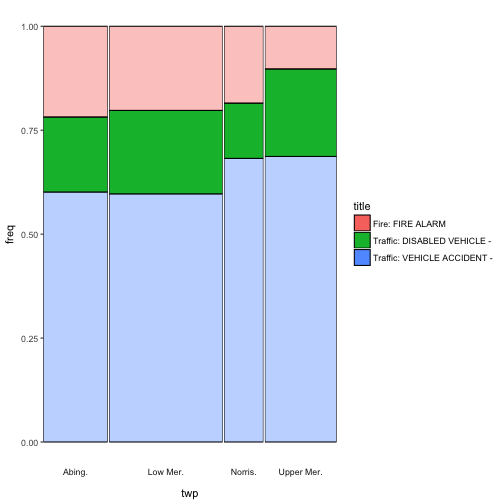
Secondly, the alpha_condition argument takes an unevaluated expression in terms of the column names of x and y. The cells for which the expression yields TRUE will be highlighted (or rather the others will be downlighted). This is useful when you want to stress an aspect of the distribution, like a value of y that varies greatly over x.
ggmm(em_sel, twp, title,
     alpha_condition = title == "Traffic: DISABLED VEHICLE -")
I hope you find this function useful. The source code is shared below. Also it is in the package accompanying this blog. Which you can install by running devtools::install_github("EdwinTh/thatssorandom").
library(tidyverse)
ggmm <- function(df,
                 x,
                 y,
                 alpha_condition = 1 == 1,
                 add_text        = c(NA, "n", "prop", "perc"),
                 round_text      = 2) {
  stopifnot(is.data.frame(df))
  add_text <- match.arg(add_text)

  x_q <- enquo(x)
  y_q <- enquo(y)
  a_q <- enquo(alpha_condition)

  plot_set <- df %>%
    add_alpha_ind(a_q) %>%
    x_cat_y_cat(x_q, y_q) %>%
    add_freqs_col()

  plot_return <- mm_plot(plot_set, x_q, y_q)

  plot_return <- set_alpha(df, plot_return, a_q)

  if (!is.na(add_text)) {
    plot_set$text <- make_text_vec(plot_set, add_text, round_text)
    plot_set$freq <- calculate_coordinates(plot_return)
    text_part <- geom_text(data = plot_set, aes(label = text))
  } else {
     text_part <- NULL
  }

  plot_return + text_part
}

add_alpha_ind <- function(df, a_q) {
  df %>%
    mutate(alpha_ind = !!a_q)
}

x_cat_y_cat <- function(df, x_q, y_q) {
  df %>%
    mutate(x_cat = as.character(!!x_q),
                  y_cat = as.character(!!y_q))
}

add_freqs_col <- function(df) {
  stopifnot(all(c('x_cat', 'y_cat', 'alpha_ind') %in% colnames(df)))
  df %>%
    group_by(x_cat, y_cat) %>%
    summarise(comb_cnt  = n(),
              alpha_ind = as.numeric(sum(alpha_ind) > 0)) %>%
    mutate(freq  = comb_cnt /sum(comb_cnt),
           y_cnt = sum(comb_cnt)) %>%
    ungroup()
}

mm_plot <- function(plot_set, x_q, y_q) {
  plot_set %>%
    ggplot(aes(x_cat, freq, width = y_cnt, fill = y_cat, alpha = alpha_ind)) +
    geom_bar(stat = "identity", position = "fill", color = "black") +
    facet_grid(~x_cat, scales = "free_x", space = "free_x",
               switch = "x") +
    theme(
      axis.text.x  = element_blank(),
      axis.ticks.x = element_blank(),
      panel.spacing = unit(0.1, "lines"),
      panel.grid.major = element_blank(),
      panel.grid.minor = element_blank(),
      panel.background = element_blank(),
      strip.background = element_blank()
    ) +
    guides(alpha = FALSE) +
    labs(fill = quo_name(y_q)) +
    xlab(quo_name(x_q))
}

set_alpha <- function(df, plot_return, a_q) {
  if (mutate(df, !!a_q) %>% pull() %>%
      unique() %>% length() %>% `==`(1)) {
    plot_return +
      scale_alpha_continuous(range = c(1))
  } else {
    plot_return +
      scale_alpha_continuous(range = c(.4, 1))
  }
}

make_text_vec <- function(plot_set, add_text, round_text) {
  if (add_text == "n") return(get_counts(plot_set))
  text_col <- get_props(plot_set)
  if (add_text == "perc") {
    text_col <- round(text_col * 100, round_text)
    return(paste0(text_col, "%"))
  }
  round(text_col, round_text)
}

get_counts <- function(plot_set) {
  plot_set %>% pull(comb_cnt)
}

get_props <- function(plot_set){
  plot_set %>%
    mutate(text_col = comb_cnt / sum(plot_set$comb_cnt)) %>%
    pull()
}

calculate_coordinates <- function(plot_return) {
  ggplot_build(plot_return)$data[[1]] %>%
    split(.$PANEL) %>%
    map(y_in_the_middle) %>%
    unlist()
}

y_in_the_middle <- function(x) {
  y_pos <- c(0, x$y)
  rev(y_pos[-length(y_pos)] + (y_pos %>% diff()) / 2)
}