I am happy to share that the latest version of padr just hit CRAN. This new version comprises bug fixes, performance improvements and new functions for formatting datetime variables. But above all, it introduces the custom paradigm that enables you to do asymmetric analysis.

Improvements to existing functions

thicken used to get slowish when the data frame got large. Several adjustments resulted in a considerable performance gain. It is now approximately 6 times faster than in version 0.3.0.

Both pad and thicken used to break with noninformative errors when the datetime variable contains missing values. Both functions allow for missing values now. thicken will leave the record containing the missing datetime value where it is and will enter a missing value in the column added to the data frame. pad will move all the records with missing values in the datetime variable to the end of the data frame and will further ignore them for padding. Both functions throw a warning when the datetime variable has missing values.

New functions

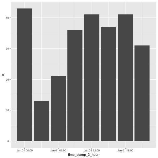
span_date and span_time are wrappers around seq.Date and seq.POSIXt and were previously described in this blog post. Two new functions are introduced to reformat datetime variable. These can be especially useful for showing the data in a plot or a graph. center_interval shifts the datetime point from the beginning of the interval to the (approximate) center. Especially bar, line and dot plots will reflect the data in a more accurate way after centering.

library(tidyverse)
library(padr)
jan_first <- emergency %>% 
  filter(as.Date(time_stamp, tz = "EST") == as.Date("2016-01-01")) %>% 
  thicken("3 hour") %>% 
  count(time_stamp_3_hour) 
ggplot(jan_first, aes(time_stamp_3_hour, n)) + geom_bar(stat = "identity")

jan_first %>% 
  mutate(ts_center = center_interval(time_stamp_3_hour)) %>% 
  ggplot(aes(ts_center, n)) + geom_bar(stat = "identity")

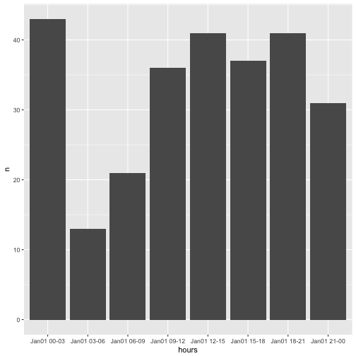
Secondly, there is the format_interval function, that will create a character from the interval using strftime on both the beginning and the end of the datetime points of each interval.

jan_first %>% 
  mutate(hours = format_interval(time_stamp_3_hour,
                                 start_format = "%b%d %H",
                                 end_format   = "%H",
                                 sep = "-")) %>% 
  ggplot(aes(hours, n)) + geom_bar(stat = "identity")

When using the interval “week”, one might want to start the weeks on different day than Sunday. In thicken the start_val should than be specified with a day of the desired weekday. Finding this day by hand is a bit tedious, thats why closest_weekday is introduced.

thicken(coffee, "week", 
        start_val = closest_weekday(coffee$time_stamp, 6))

##            time_stamp amount time_stamp_week
## 1 2016-07-07 09:11:21   3.14      2016-07-02
## 2 2016-07-07 09:46:48   2.98      2016-07-02
## 3 2016-07-09 13:25:17   4.11      2016-07-09
## 4 2016-07-10 10:45:11   3.14      2016-07-09

The custom suite

thicken and pad are highly automated, because they assume all datetime points to be equally spaced. Internally they span vectors of the desired interval. However, it might be useful to have asymmetrical periods between datetime points. Especially when there are periods in which the number of observations is consistently lower, such as nightly hours or weekend days. The functions thicken_cust and pad_cust work like the original functions. However, the user has to provide his own spanning vector to which the observations are mapped.

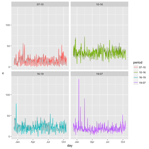
Lets do an analysis of vehicle accidents in the emergency. We want to distinguish between morning rush hour (7-10), daytime (10-16), evening rush hour (16-19) and nighttime (19-7). This is the full analysis.

accidents_span <-
  span_around(emergency$time_stamp, "hour", start_shift = "2 hour") %>% 
  subset_span(list(hour = c(7, 10, 16, 19)))

emergency %>% 
  filter(title == "Traffic: VEHICLE ACCIDENT -") %>% 
  thicken_cust(accidents_span, "hour") %>% 
  count(hour) %>% 
  pad_cust(accidents_span) %>%
  fill_by_value() %>% 
  mutate(day    = as.Date(hour, tz = "EST"),
         period = format_interval(hour, start_format = "%H", sep = "-")) %>% 
  ggplot(aes(day, n, col = period)) + 
  geom_line() +
  facet_wrap(~period)

The helper functions span_around and subset_span are used for building the spanning vector. The first takes the original datetime variable and spans a variable of the requested interval around it. This saves you the manual trouble of finding the min and the max of the variable and determine which points are respectively before and after them to build a variable of the interval. subset_span, subsequently, will only leave the datetime points in the input that meet the criteria given in a list. In the example these are the hours 7, 10, 16, and 19. In total there are eight different datetime parts you can subset on.

The remainder of the analysis is greatly similar to a regular padr analysis. Instead of an interval to which to thicken and pad to, you use the asymmetrically spaced accidents_span variable in both thicken_cust and pad_cust. thicken_cust will then map each observation to a datetime point in the spanned vector. pad_cust will insert rows for each of the observations that are in the spanned vector, but not in the datetime variable.

Thanks

This release completes the initial plans I had for padr. For the next release I plan on refactoring and further increasing performance. Do you find anything still missing from padr? Did you find a bug or an inconsistency? Please notify by sending an email or file an issue on the github page.